accelerated gossip
Accelerated Gossip in Networks of Given Dimension using Jacobi Polynomial Iterations by Raphaël Berthier, Francis Bach and Pierre Gaillard
Final project for MAP578 course (Emerging Topics in Machine Learning: Collaborative Learning) at École Polytechnique. Paper study and implementation. Group project with Marc Boëlle and Antoine Millet.
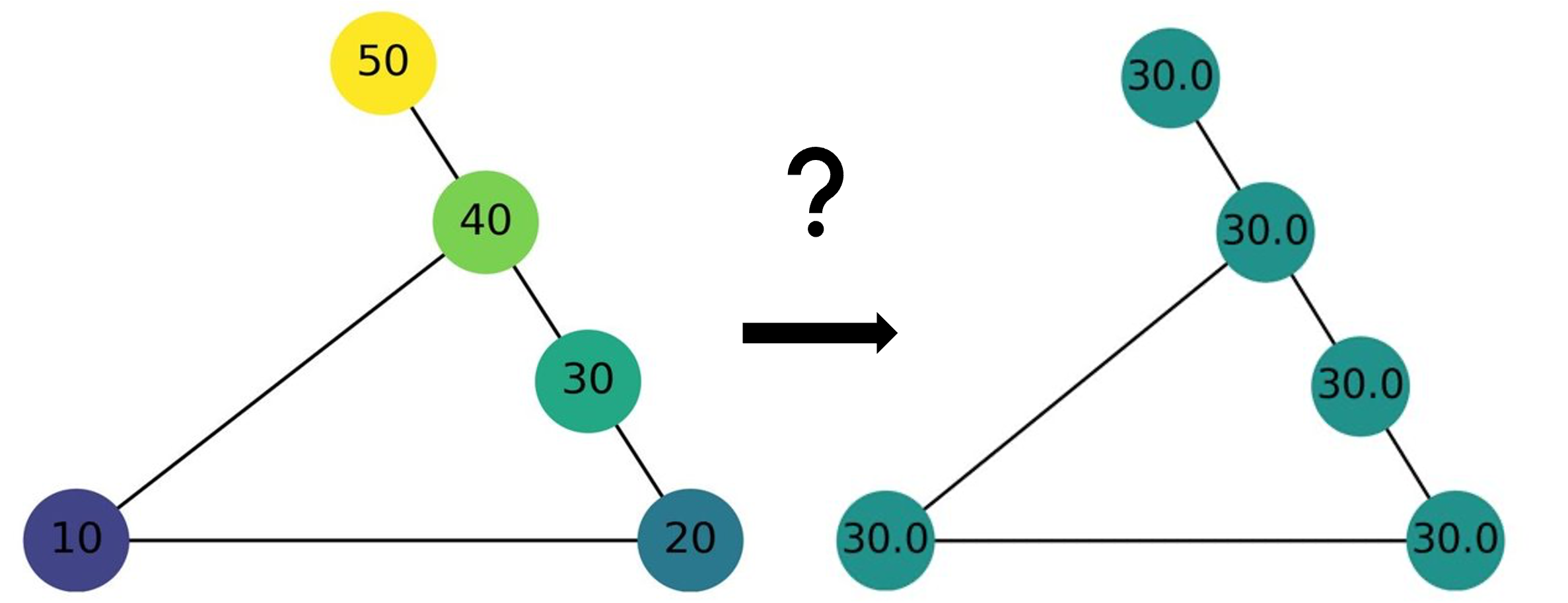
Gossip problem framework: Given a network of agents represented as a graph, in which each agent holds a real value, we want to estimate the average of these values in a distributed manner. The agents (nodes) are related through links (edges), which they can use to communicate.

Overview : The authors build a method for solving this problem that depends only on what they define as the spectral dimension of the network, which is intuitively the dimension of the space in which the agents live (for a grid in \(\mathbb{Z}^n\), the spectral dimension is \(n\)). Their method shows improvement over previous algorithms in the non-asymptotic regime, when the values are far from fully mixed.
The gossip problem and gossip algorithms
The gossip problem
The gossip problem, also known as the averaging problem, is fundamental in distributed networks, when information is shared among several machines without a central server. In this framework, we assume that each machine can communicate only with a few others, and these links are represented in a graph \(G=(V,E)\). Each machine hold an initial real value that the others do not know. The goal is then to find a way to get each machine to know the average of these initial values, through an iterative communication procedure and as quickly as possible.
Problem Setting
We are given an undirected finite graph \(G=(V,E)\), where \(V\) is the set of agents (nodes) in the network, and \(E\) the set of communication links (edges). Each node \(v\in V\) receives an initial real value \(\xi_v\) called an observation. We denote by \(\xi=(\xi_v)_{v\in V}\) the vector of observations, and the goal is then for each machine to know \(\bar\xi=\frac{1}{|V|}\sum_{v\in V}\xi_v\) through an iterative algorithm.
\(x^t=(x^t_v)_{v\in V}\) denotes the values at time \(t\).
NB : we are in in a synchronous framework, meaning that at every time step, all communciations are made at the same time (and not successively)
Simple gossip algorithm
Referred to as simple gossip in the paper, the landmark algorithm consists in the following intuitive scheme: at each iteration, each agent replaces his current value by an average of the values held by its neighbors. Formally, this means that we have a gossip matrix \(W\), which is stochastic, symmetric, nonnegative and supported by the graph : \(W_{u,v}>0\implies \{u,v\}\in E\).
usual gossip matrix
If all vertices have degree smaller than \(d_{\max}\): \(W=I+\frac{1}{d_{\text{max}}}(A-D)\)
Then the simple gossip algorithm consists in the updates \(x^{t+1}=Wx^t\), leading to \(x^t=W^t\xi\).
Shift-register gossip algorithm
The idea of this second gossip algorithm is to take a linear combination of past iterates : \(x^{t+1}=\omega Wx^t+(1-\omega)x^{t-1}\) with \(x^0=\xi\) and \(x^1=W\xi\) Without going into the details of this algorithm, it is clear that the parameter \(\omega\) plays an important role and must be finetuned.
It was shown in
This is a nice improvement since \(\gamma\) is indeed very small in large graphs. And in practicle cases, graph networks are quite big, so it is a worthy improvement.
Yet one important point here is that we assume that all agents know the spectral gap \(\gamma\). But in the general case, there is no reason why they should. Thus, the point of this paper is to find a way to avoid this difficulty by building a method based not on \(\gamma\) but on the spectral dimension of the graph.
Polynomial gossip
Intuitively, polynomial gossip consists in replacing \(x^t=W^t\xi\) by \(x^t=P_t(W)\xi\). In other words, at every time step, we take linear combinations of all past iterates of the simple gossip method.
The polynomials consider must verify \(\text{deg}P_t\leq t\) (to ensure that the \(x^t\) can be computed using at most \(t\) communication steps) and \(P_t(1)=1\) (to ensure that if all initial observations are equal, then \(x^t=\xi\) for any \(t\)).
Diagonalizing \(W\), with \(1=\lambda_1>\lambda_2>\lambda_n>-1\), the simple gossip formula can be rewritten as :
\[x^t = U \begin{pmatrix} 1 & 0 & \cdots & 0 \\ 0 & \lambda_2^t & \cdots & 0 \\ \vdots & \vdots & \ddots & \vdots \\ 0 & 0 & \cdots & \lambda_n^t \end{pmatrix} U^T \xi\]And same for the polynomial gossip formula:
\[x^t = U \begin{pmatrix} P_t(1) & 0 & \cdots & 0 \\ 0 & P_t(\lambda_2) & \cdots & 0 \\ \vdots & \vdots & \ddots & \vdots \\ 0 & 0 & \cdots & P_t(\lambda_n) \end{pmatrix} U^T \xi\]Finding the optimal polynomials
Error to measure performance
\[\mathcal{E}(P_t)=\|x^t-\bar\xi 1\|^2=\|P_t(W)\xi-\bar\xi 1\|^2\] \[\mathcal{E}(P_t)=\int_{-1}^1P_t(\lambda)^2d\sigma (\lambda)\]with \(d\sigma (\lambda)=\sum_{i=2}^n\langle\xi,u^i\rangle^2\delta_{\lambda_i}\) the spectral measure
Optimization
We want to find \(\pi_t\) such that:
\[\pi_t\in\underset{P_t(1)=1,\deg P_t\leqslant t}{\text{argmin}}\mathcal{E}(P_t)\]So the optimal polynomial \(\pi_t\) verifies:
\[\pi_t\in\underset{P_t(1)=1,\deg P_t\leqslant t}{\text{argmin}}\int_{-1}^1P_t(\lambda)^2d\sigma (\lambda)\]Final goal : minimize this error, under the conditions on degree and value in 1.
Some results on orthogonal polynomials
theorem: orthogonal polynomials
\(\pi_t\) is unique and \(\pi_0,\pi_1,\dots\) is the unique sequence of orthogonal polynomials w.r.t. \(\tau\) defined as follows, and normalized such that \(\pi_t(1)=1\) :
\[d\tau(\lambda)=(1-\lambda)d\sigma(\lambda)\]theorem: second order recursion
Let \(\pi_0,\pi_1,\dots\) be a sequence of orthogonal polynomials w.r.t. some measure \(\tau\). There exist three sequences of coefficients \((a_t)\), \((b_t)\) and \((c_t)\) such that :
\[\pi_{t+1}(\lambda)=(a_t\lambda+b_t)\pi_t(\lambda)-c_t\pi_{t-1}(\lambda)\]We know that our optimal polynomial \(\pi_t\) minimizes this integral w.r.t. the spectral measure sigma
Now we know from the theorem above that \(\pi_t\) defined as such is unique, and that the sequence \(\pi_0, \pi_1\cdots\) is the unique sequence of orthogonal polynomials wrt the measure \(\tau\) defined here, and normalized to satisfy our condition of value in 1
We won’t need to know much about orthogonal polynomials, except that they always follow a second order recursion (see theorem above) with coefficients \(a_t,b_t,c_t\).
Back to gossip
Thus we get the following formula :
\[x^t=\pi_t(W)\xi\]And from the second order theorem :
\[\begin{align*} &x^{t+1} = a_t W x^t + b_t x^t - c_t x^{t-1} \\ &x^1 = a_0 W \xi + b_0 \xi \\ &x^0 = \xi \end{align*}\]Conclusion: the best polynomial gossip algorithm is a second order method. This is good in practice, because it implies a limited memory cost to store past values.
Problem : the polynomials are hard to compute because the spectral measure \(\sigma\) is unknown in pratice. So the idea is to approximate \(\sigma\) with a simpler measure \(\tilde\sigma\). => How do we choose \(\tilde\sigma\) ?
Approximating the spectral measure
Based on the notion of spectral dimension introduced in the paper
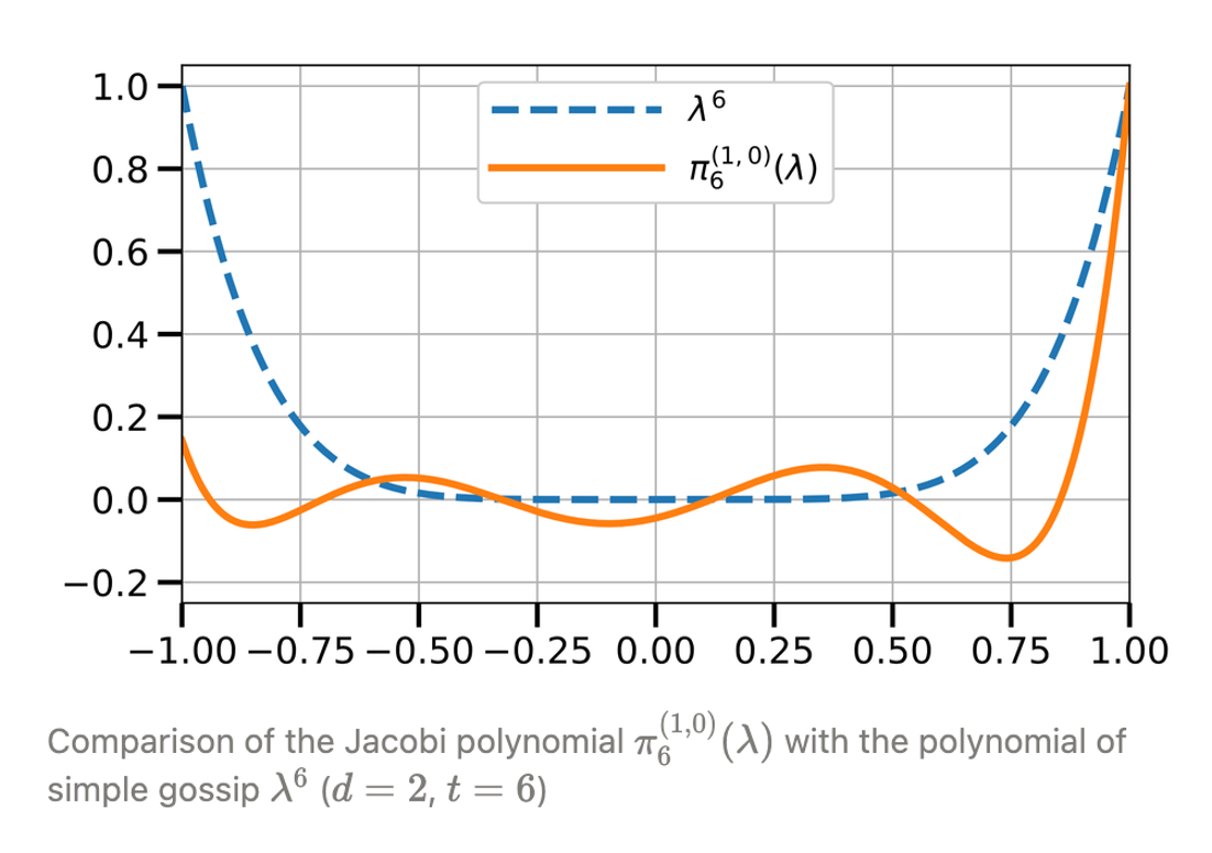
With the \(\tau\) notation previously introduced for orthogonal polynomials, we end up having to determine the sequence of orthogonal polynomials associated to the following measure: \(d\tilde{\tau}(\lambda) = (1 - \lambda)^{d/2} \mathbb{1}_{\{\lambda \in (-1,1)\}} \, d\lambda\)
And this sequence turns out to be the Jacobi polynomials!

formulas for the coefficients of the Jacobi polynomials
\[\begin{align*} a_0^{(d)} &= \frac{d + 4}{2(2 + d)}, \\ a_t^{(d)} &= \frac{(2t + d/2 + 1)(2t + d/2 + 2)}{2(t + 1 + d/2)^2}, \\ c_t^{(d)} &= \frac{t^2(2t + d/2 + 2)}{(t + 1 + d/2)^2(2t + d/2)}, \\ b_0^{(d)} &= \frac{d}{2(2 + d)}, \\ b_t^{(d)} &= \frac{d^2(2t + d/2 + 1)}{8(t + 1 + d/2)^2(2t + d/2)}. \end{align*}\]Simulations
Moving on to simulations, we systematically compared the performances of the different methods we’ve presented : simple gossip, shift-register, and Jacobi iterations. We decided to focus on 2-dimensional grids, and to visualize them as images in which each pixel represents a node and its color represents the value it holds.
Normal distribution
For the initial distribution, the authors decided to use only \(\xi\sim\mathcal{N}(0,1)\). So we decided to first see how the algorithms performed on this distribution, and then to try them on a completely different one.
First with the normal distribution, we can see indeed that the Jacobi method converges faster than the other two.
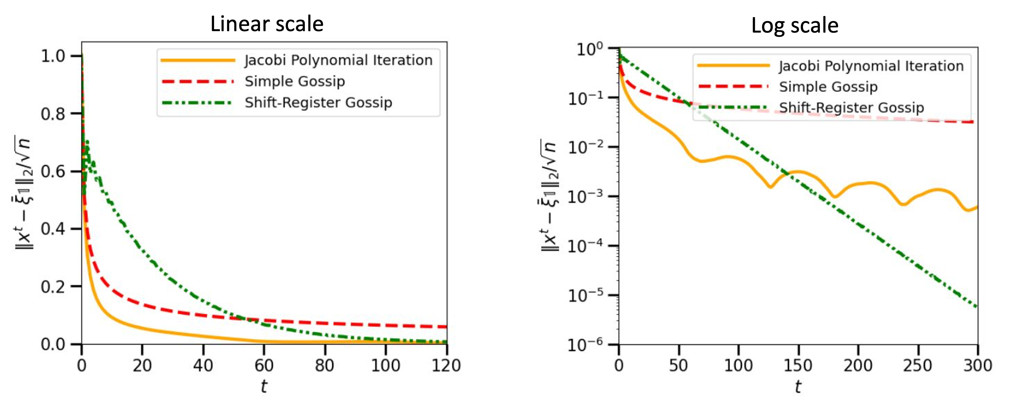
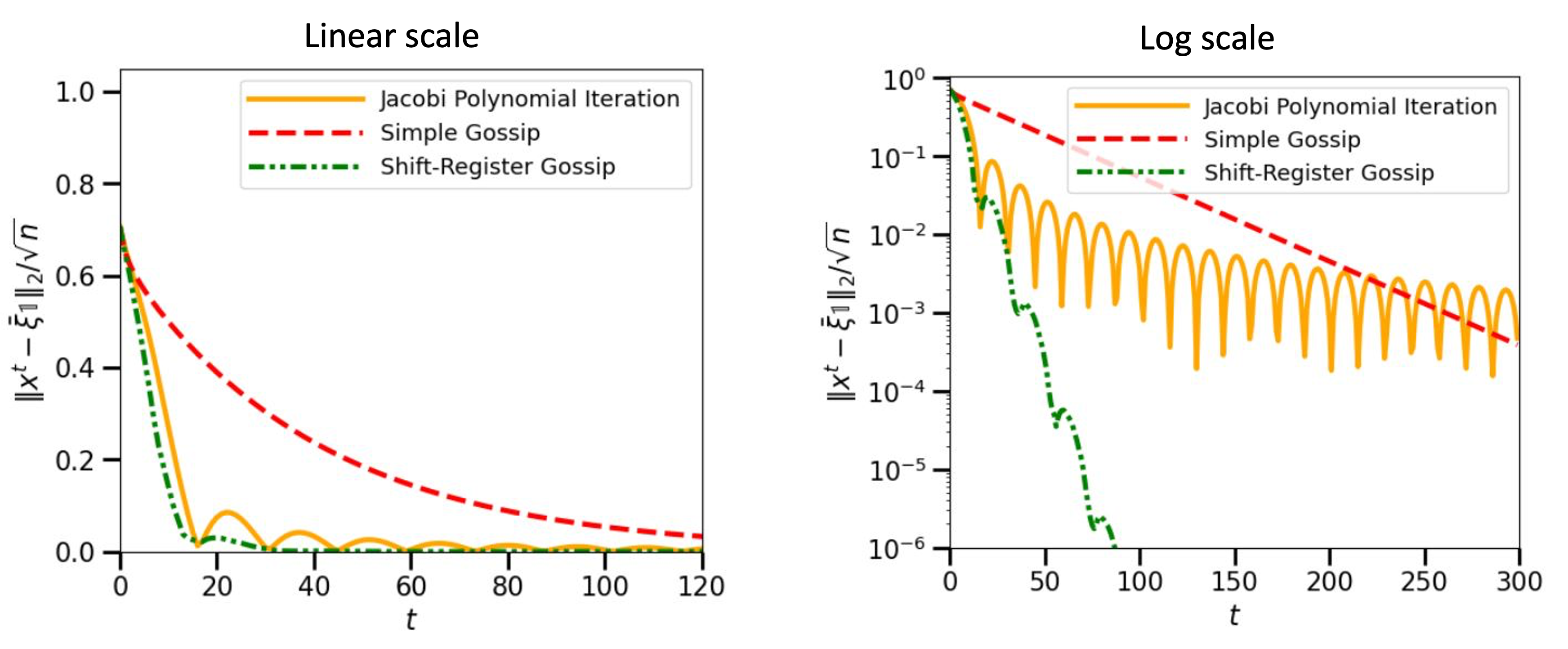
To evaluate performance more precisely, we plotted the error as a function of time, both in linear and log scale :

The log scale provides a more precise understanding of the error : Jacobi is best at first, and then shift-register achieves better results, but this is when the error is already very small (\(10^{-3}\)) after many iterations. In practical cases we won’t necessarily need this extra precision, so fast convergence in short term will often be good enough.
Step distribution
