fairness with Wasserstein barycenters

Fair Regression with Wasserstein Barycenters by Evgenii Chzhen, Christophe Denis, Mohamed Hebiri, Luca Oneto, and Massimiliano Pontil

Final project for MAP588 course (Emerging Topics in Machine Learning: Optimal Transport) at École Polytechnique. Paper study and implementation. Group project with Marc Boëlle and Martin Morange.

Results of the paper

Problem setting

The authors focus on regression problems \(Y=f^*(X,S)+\xi\), where \(f^*\) is the regression function minimizing the squared risk, \(S\) a sensitive attribute and \(\xi\) a (centered) noise.

Demographic Parity (DP)

To evaluate the fairness of some predictors, there are different metrics available. Demographic Parity is one of them and extensively used in the literature, in particular in this paper. Intuitively, it is satisfied if the distribution of the prediction is independent of the sensitive attribute.

Formally, with \(S\) the attribute representing the sensitive groups in the population, a predictor \(g\) is fair (according to the DP criterion) if

\[\forall (s,s')\in S^2,\:\:\sup_{t\in\mathbb{R}}\left|\mathbb{P}(g(X,S)\leq t|S=s)-\mathbb{P}(g(X,S)\leq t|S=s')\right|=0\]

In other words, the Kolmogorov-Smirnov distance between the distributions on all sensitive groups must be \(0\).

Strategy of the authors

From the optimal predictor \(f^*\), the authors suggests that we build a fair predictor \(g^*\) (w.r.t. DP) which remains “close” to \(f^*\) - to keep the accuracy as high as possible. We end up with this new problem :

\[\min_{g\text{ is fair}}\mathbb{E}\left(f^*(X,S)-g(X,S)\right)^2\]

Using Optimal Transport theory, the authors provide a closed form expression of \(g^*\) using Wasserstein barycenters :

Theorem:

\[\min_{g \text{ is fair}} \mathbb{E}(f^*(X,S) - g(X,S))^2 = \min_{\nu} \sum_{s \in S} p_s \mathcal{W}_2^2(\nu_{f^*|s}, \nu)\] \[g^*(x,s) = \left( \sum_{s' \in S} p_{s'} Q_{f^*|s'} \right) \circ F_{f^*|s}(f^*(x,s))\]

with

\[\mathcal{W}_2^2(\mu, \nu) = \inf_{\gamma \in \Gamma_{\mu, \nu}} \int_{\gamma \in \Gamma_{\mu, \nu}} |x - y|^2 d\gamma(x,y)\]

with $$F_{f

s}\(the CDF of\)f\(,\)Q_{f

s}\(its quantile function and\)p_s = \mathbb{P}(S=s)$$.

Insurance dataset

Data visualization

The first dataset we worked on is the insurance dataset. Each row corresponds to an individual, and our goal is to predict the amount of charges people have to pay for medical insurance. The sensitive groups we chose to consider for fairness evaluation are smokers and non-smokers. You may guess that smokers will have to pay higher charges for medical insurance than non-smokers. And indeed they do:

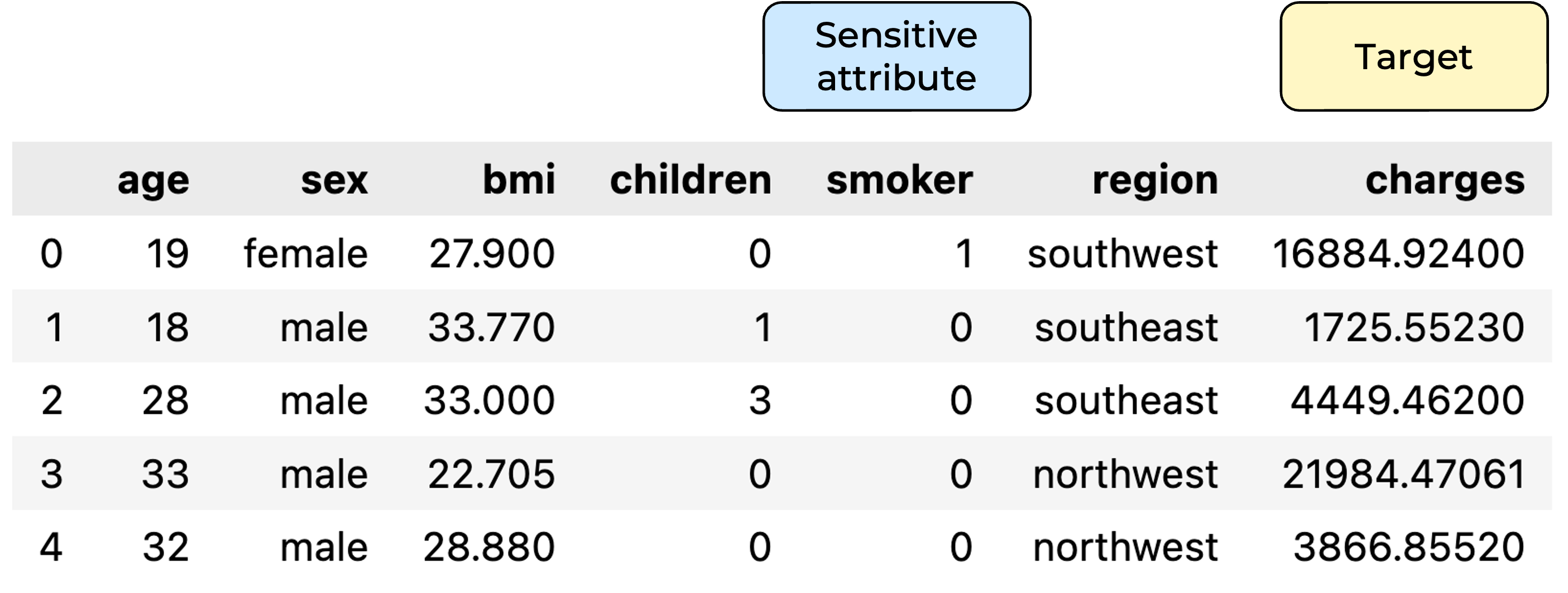
Of all the plots we made to visualize the data, we liked the following one :

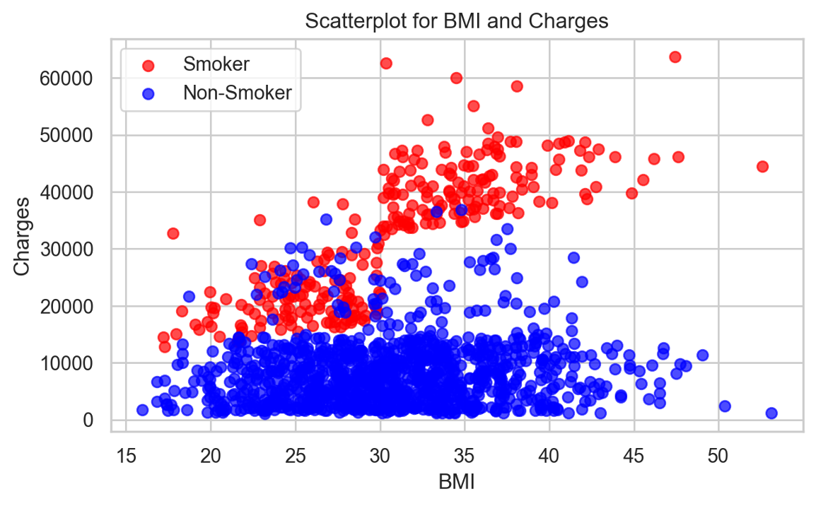
It’s a scatter plot for charges versus BMI (Body Mass Index), and we’ve colored the points according to the sensitive attributes – smokers are in red, and non-smokers are in blue. You can clearly see the bias in the data, the red points being mostly above the blue ones. And we especially liked this plot because it also shows another bias, which is that the smokers who pay the highest charges are those with a large BMI. But for our study we’ll focus only on the fairness regarding the groups of smokers and non-smokers. Then, with this huge bias, we were curious to see how good the algorithm from the paper would be at making a predictor fair.

Training a first unfair predictor

What we needed first was a base predictor, and to get one we used simple Machine Learning models from scikit-learn.

To compare the performances of these models, we used RMSE, which stands for Relative Mean Squared Error, and is defined as such : take the mean squared error of your predictor, and divide it by the variance of the groundtruth labels (which is in other words the mean squared error you would get with a predictor that always predicts the average of the groundtruth labels).

\[\text{RMSE}\:(g)=\frac{\displaystyle\sum_{(x,y)\in\mathcal{D}}(y-g(x))^2}{\displaystyle\sum_{(x,y)\in\mathcal{D}}(y-\overline{y})^2}\]

With this error function, the best model we found is a gradient boosting regressor, which gave us an RMSE of 0.34.

Building the fair predictor

Now that we have this base model, we can move on to building the fair predictor using the post-processing algorithm from the paper .

Then, to evaluate fairness, we use the Demographic Parity distance defined earlier : the maximum difference between the CDFs on each sensitive group.

\[DP(g;s,s')=\sup_{t\in\mathbb{R}}\left|\mathbb{P}(g(X,S)\leq t|S=s)-\mathbb{P}(g(X,S)\leq t|S=s')\right|\]

So a fair predictor will have a DP distance close to zero, meaning that the CDFs will be the same for the different sensitive groups. And the link with CDFs gives us a good way to visualize fairness.

Results

So we plotted the empirical CDFs of the predictions on the two sensitive groups separately (smokers and non smokers).

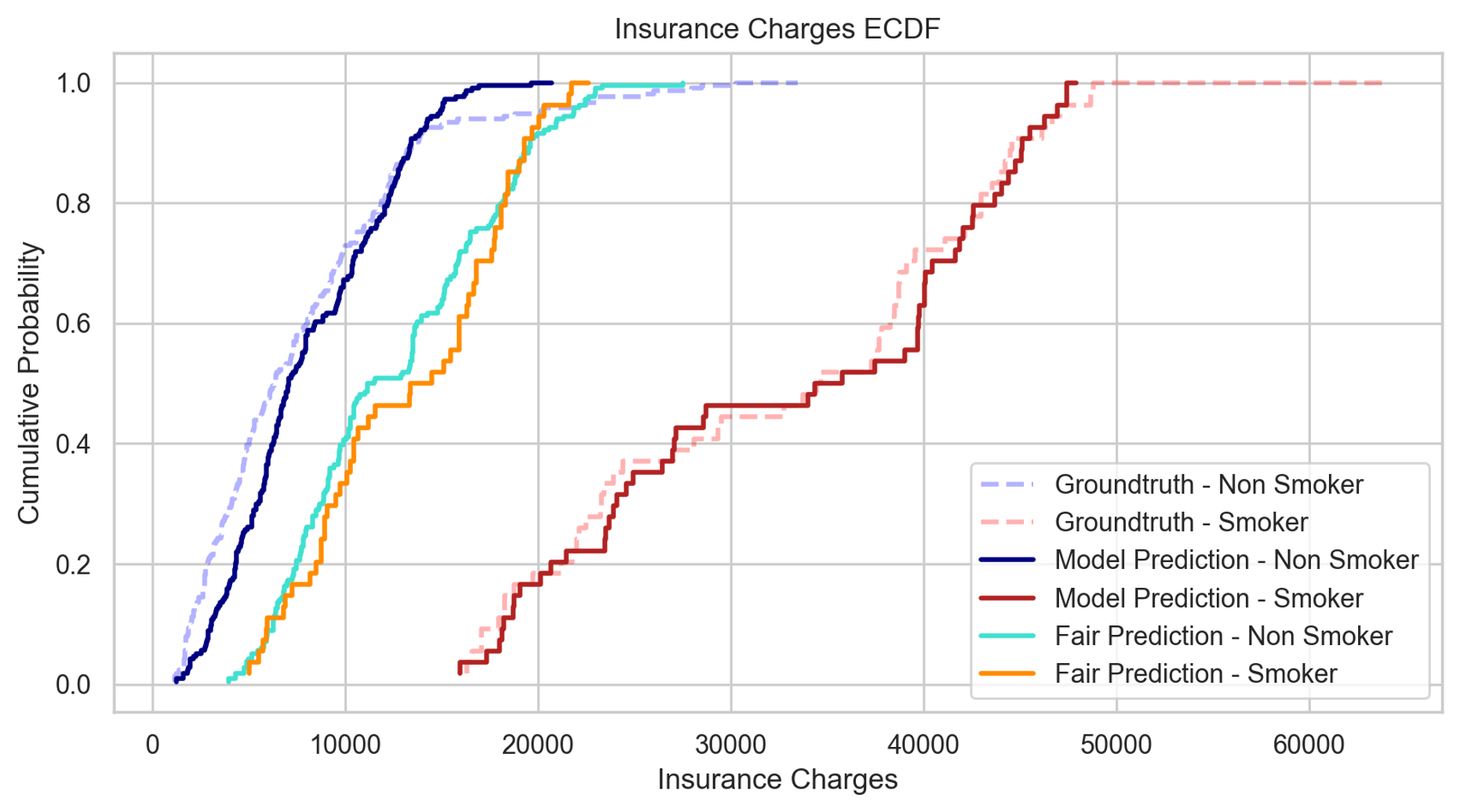
In dark blue and dark red, we have the ECDFs for the base model predictions, respectively for non smokers and smokers : we can see that the DP distance is close to 1, meaning that this predictor is very unfair. This is normal since it was trained on highly biased data. Then, in light blue and orange, we have the ECDFs for the post-processed model predictions, respectively for non smokers and smokers : they are much closer to one another, the distance is around 0.2, so we did gain a lot of fairness. But we can see that the blue curve remains mostly above the orange one, meaning that the predictor is still biased.

Now, seeing this plot, we wondered what would happen if we made an interpolation between those two states, how it would impact fairness.

Interpolation

So that’s we did next, we made a simple linear interpolation between the model predictions and the post-processed predictions, with a parameter alpha representing the weight given to the fair predictions.

(1 - alpha) * predictions + alpha * fair_predictions

What we expected from the paper was to reach optimal fairness at alpha=1 (because that’s what theory says).

But given the remaining bias we saw on the previous plot, we were also curious to see what would happen for alpha larger than 1, if we pushed the interpolation a bit further.

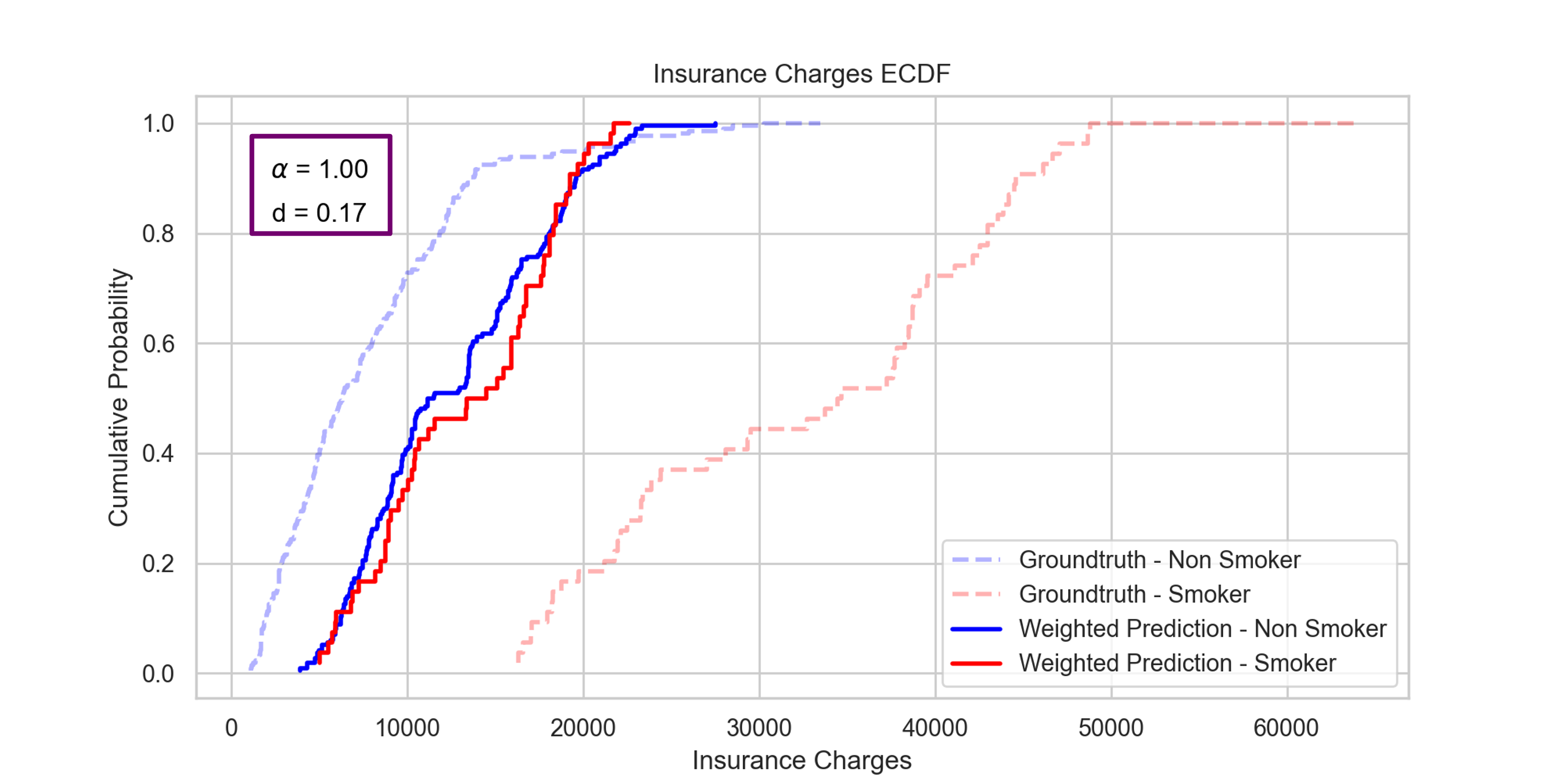
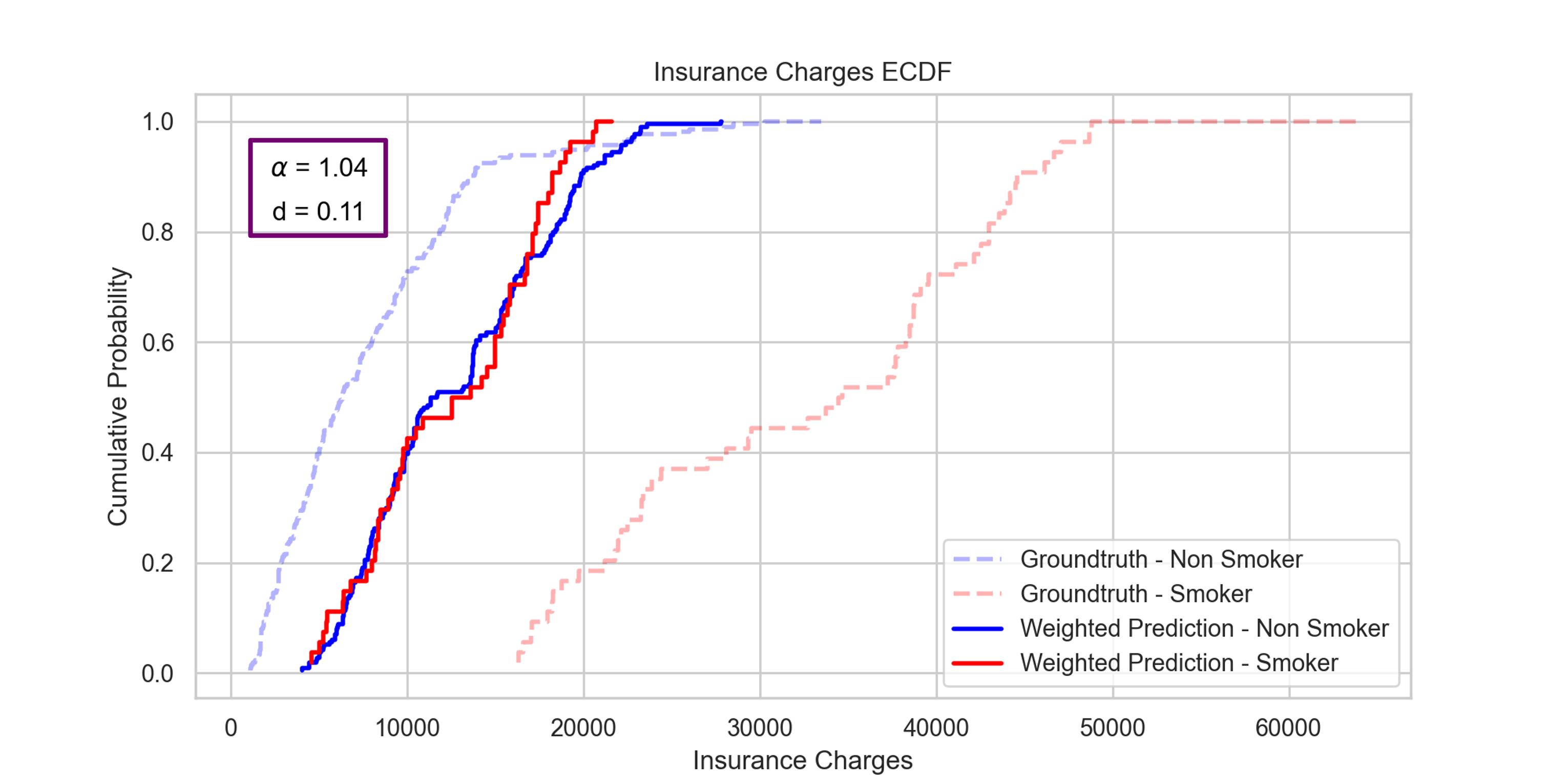
that’s what we did, and we found out that optimal fairness was reached for alpha larger than one : indeed, we get a DP distance of 0.17 with alpha=1, and 0.11 with alpha=1.04, which is the optimal value.

Fairness vs. Accuracy

Finally, to better see what happens, we plotted the DP distance versus the RMSE, colored by the value of alpha :

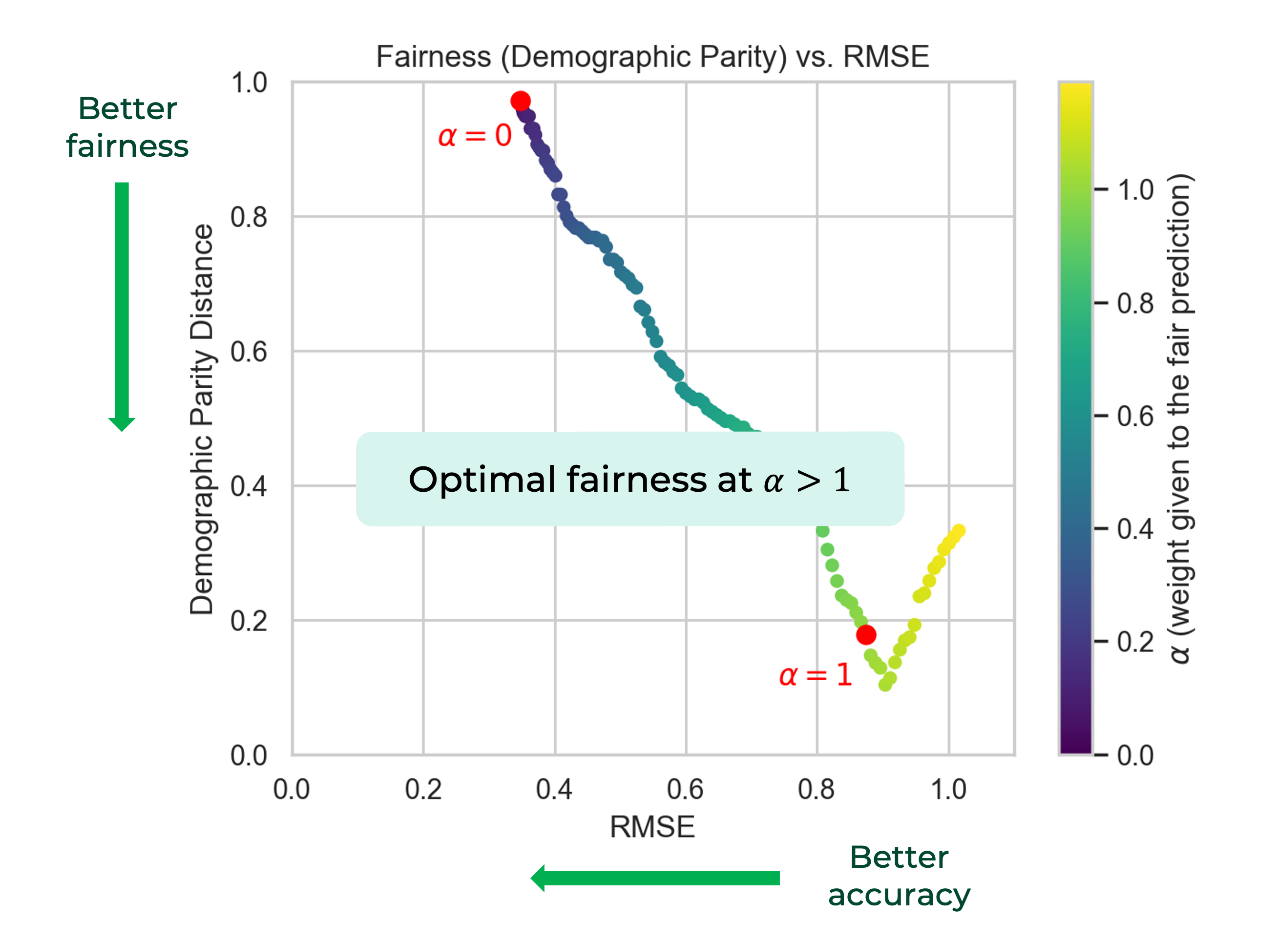
first we see that when improving fairness (going down the y axis), we loose accuracy - which we expected.

But also, you can clearly see here that alpha=1 is not optimal, and that the fairness distance keeps decreasing a bit, before going up again.

This was not discussed in the paper at all, and we believe there could be further experiments to have a deeper understanding of what happens here.

So now that we’ve seen our results on this first dataset with a very strong bias, I’ll let Martin take over for the results on our second dataset which is quite different.

Income dataset

Data visualization

Goal : predict the salary Groups considered for fairness evaluation : male and female

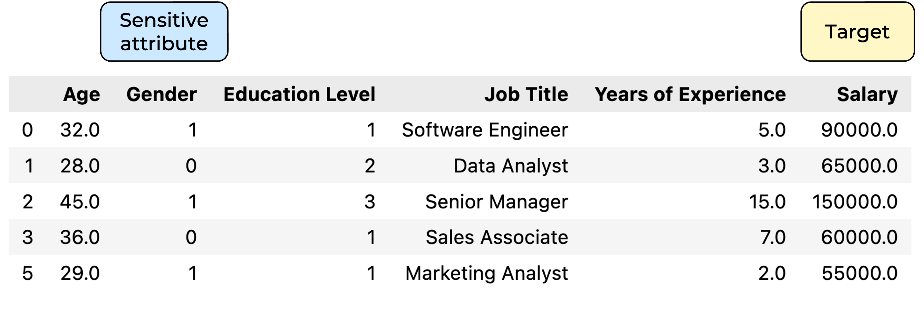
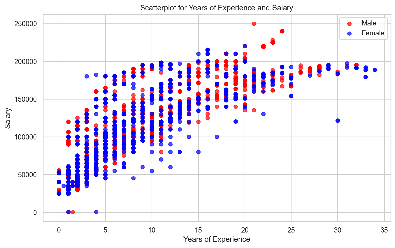
The data is still biased, but less biased than in the insurance dataset

Let’s see how it impacts fairness of the predictor

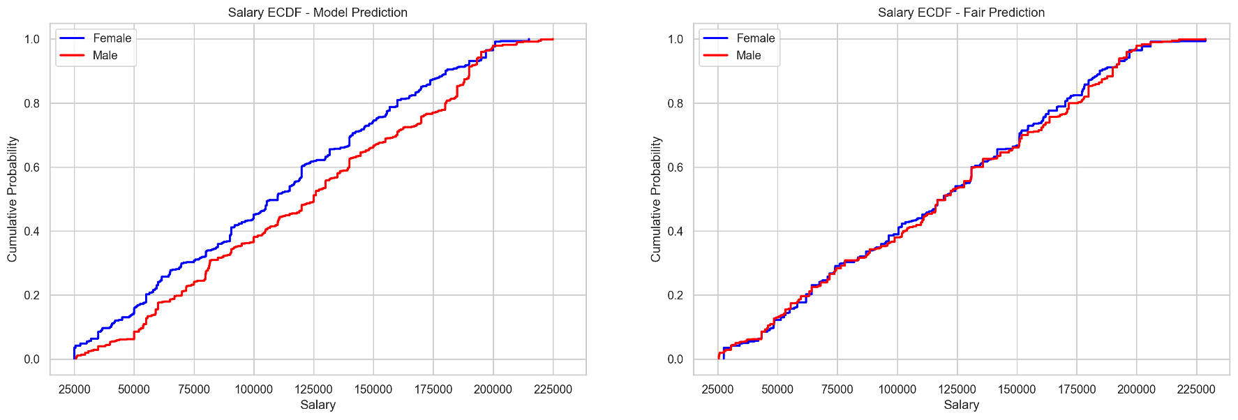
Model predictions are fairer than on the insurance dataset, and the postprocessing seems to achieve better final fairness

Conclusion

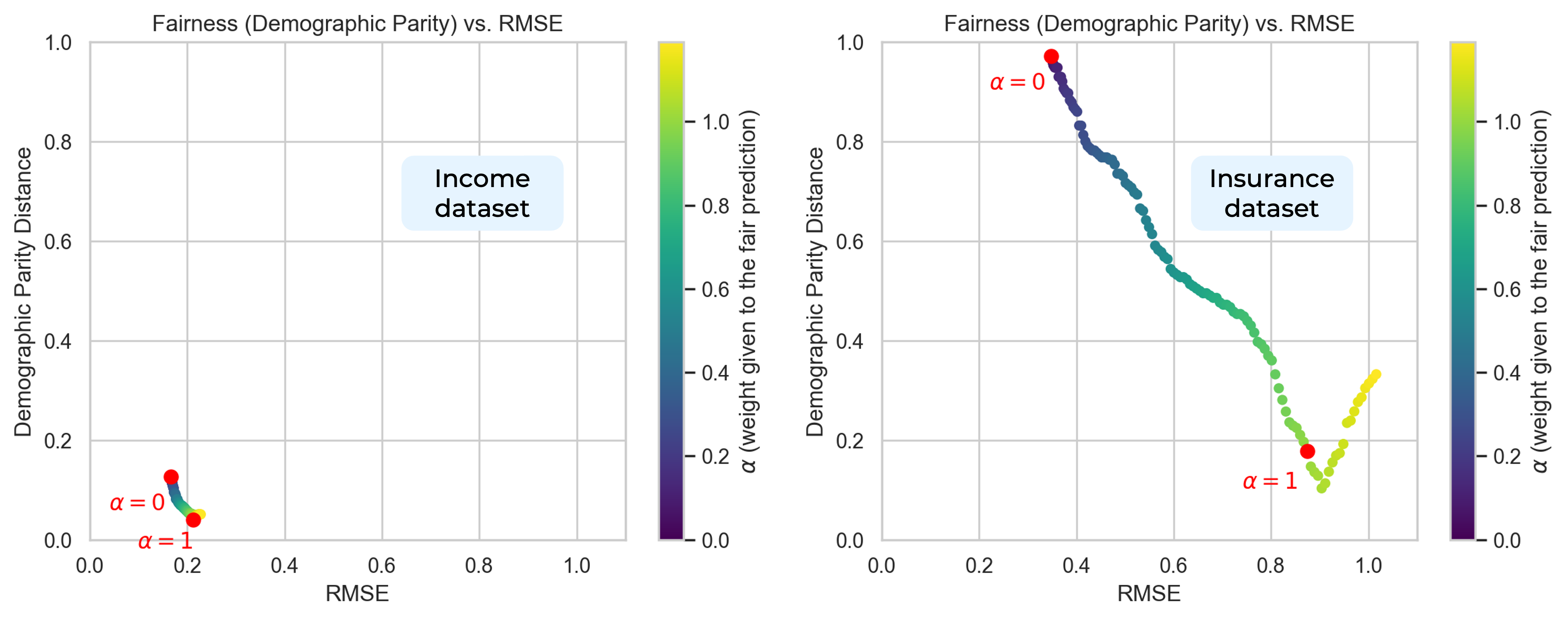
trade-off accuracy vs. fairness